DSW (DAY, STOUT & WARREN) ALGORITHM

DSW (DAY, STOUT & WARREN) ALGORITHM 

DSW algorithm is one of the most elegant techniques available to balance a tree globally. Global tree balancing happens when all the operations such as insertions and deletions on a tree is completed. So unlike AVL trees where a rebalance (local) occurs each and every time the height difference is ±2 this algorithm works on a tree which has no pending operations and not as a part of the insert or delete operation as in the AVL tree. This algorithms always creates trees that are perfectly balanced or close to being perfectly balance.

The DSW algorithm has two major phases and each phase is dominated by tree rotations. The steps are given below

1) Create Backbone 

2) Create the Balanced Tree

Let discuss these steps in detail taking the tree in Figure 1 as our example.

Figure 1: Binary Search Tree 

Create Backbone (Vine) 

This is the initial step of the DSW algorithm. What it does is that it transforms a given tree in to a linked list like tree which is called the backbone or a vine. The pseudo code for this phase of the algorithm is given below.

Funtion CreateVine(Node root){

        tmp = root; 

        while(tmp != null){ 

                if( tmp has leftChild) 

                            right rotate leftChild around tmp 

                            update tmp to the child which just became parent                  else

                            tmp = tmp.right

             }

}

Now lets process the tree in Figure 1 according to the above mentioned pseudo code. We initialize tmp variable to the root which at the beginning is 20. Since tmp has a left child (15) a right rotation is performed around its parent which is 20. The resulting tree is given figure 2 (a). Also note now the tmp variable points to 15.

Figure 2: Steps of the create vine phase (steps 2 & 3)

Now since tmp is at 15 and it does not have a left child it moves down the right subtree to 20. Now 20 has a left child (Figure 2 (b)) which is 17. Therefore 17 has to be right rotated about its parent 20 and tmp is updated to point to 17. Figure 3 (a) depicts the state of the tree after the right rotation of 17.

Figure 3: Steps of the create vine phase(steps 4 & 5)

Since tmp (17, Figure 3 (a)) does not have a left child tmp move to its right child and now points to the node containing the value 20 (Figure 3 (b)). Since the node 20 has a left child a right rotation is performed on the left child (19) about its parent 20. This is shown in Figure 4 (a). Now since 19 does not have a left child the tmp move to its right child and now points to 20 (Figure 4 (b)).

Figure 4: Steps of the create vine phase(steps 6 & 7)

The process keeps on going until the tmp becomes null. This will only happen once tmp has gone beyond the node 50. Once the create vine process terminates the final state of the tree is given in figure 5.

Figure 5: Vine created by the create backbone phase

The best case is when the tree is like the one in figure 5 where no rotations are required. The worst case is the mirror image of figure 5 where the loop executes 2n-1 times and perform n-1 rotations along the way. However the run time of the initial phase is O(n).

Create Balanced Tree

This is the final phase of the DSW algorithm. This phase converts the vine created in the initial phase to a perfectly balanced tree or a one that has leaf node at two adjacent levels of the tree. A perfectly balanced tree is one which has all its leaf nodes at the same level. This represents and exact triangle. Which means a relationship can derived between the height (h) of the perfectly balanced tree and the total number of nodes (n) in the tree. Therefore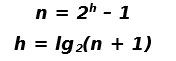

Since we know the number of nodes in the tree using the 2nd equation above the height of a perfectly balanced tree  to the corresponding number of nodes can be found. Since the vine in figure 5 contains 9 nodes the closest height of a perfectly balanced tree is 3 ( lg2(10) ~ 3). So the number nodes (m) in a perfectly balanced tree of height 3 as per the 1st equation above is 7.

n = number of nodes in the tree to be balanced (9 nodes)
m = number of nodes in the closest perfectly balanced tree (7 nodes)


So the node difference between the perfect tree and the tree to be balanced can be calculated by n-m which results in 2. This is called the excess of nodes to the perfectly balanced tree. In order to do away with this access node left rotation is performed on every second node of the vine in figure 5. Every second node is shown in green in figure 5. So m-n rotations which is 2 are performed initially to cover up the excess. Resulting tree is given in figure 6 and the updated every 2nd nodes are given in purple. The initial m-n rotations will never reach the end of the vine it terminates in the middle. The resulting tree in figure 6 has a modified vine of 7 nodes. This is equal to the number of total nodes in the perfectly balanced tree which was considered for m-n calculations.

After the preprocessing step mentioned above left rotations are performed to each every second node of the vine halving the size of the vine through each pass. Number of rotations to be performed is calculated by m which is halved in each iteration of the loop as m = m/2 (only take the integer value). So to start the final phase we recalculate m which is (7/2 = 3). So 3 left rotations are performed to the vine in figure 6. The resulting tree after the three rotations are given in figure 7.

Figure 6: Vine after n-m rotations

Figure 7: Vine after the 3 rotations

In the next iteration m further halved to 1. So one left rotation is performed on the second node in the vine. The resulting tree is shown in figure 8.

Figure 8: Final tree after the DSW algorithm

If m was further divided the value will be lesser than 1. Therefore the height differences is now less than one or one. Therefore the tree has attained a balanced state. So the tree in figure 8 is the final globally balanced tree. Observe that all the leaf node are at level L or L-1. The pseudo code of the create balanced tree phase is given below.

Function CreateBalancedTree(int  numOfNodes){ 

           int m = 2^(lg2(numOfNodes + 1)) – 1; 

           make n – m right rotations 

           while (m > 1)             //tree has not attained a balanced state 

                       m = m/2 

                       make m left rotations starting from the top of the                               back bone 

}

Also note that the above discussion is based on that the vine is created to the right as in figure 5. The vine can also be created to the left but the algorithm should also change accordingly.